Back to Basics: Optimize your search parameters
Every now and then you need to determine good search parameters for a data set. They may be different from the normal ones you use due to a change in instrumentation, you may be analyzing data from a public resource like PRIDE/Proteome exchange or it could be data from a collaborator. Whatever the reason, here’s a quick overview on how to choose some basic search parameters for a data set. If you are completely new to database searching, I recommend reading the tutorial first as it covers many of the key concepts.
For these examples, I used the wild type data from PRIDE Project PXD004560 “Pseudomonas aeroginosa resistant against Ciprofloxacin” and the Pae_wt_20151107_1.raw data file as the individual test file.
1. Pre-search investigation
If the data set is published, a quick read of the paper or the PRIDE project page should clear up anything unusual about the sample. In particular, you are looking for the following bits of information: species; alkylation method; digestion enzyme; instrument type; fragmentation method. You need to check to see if the sample is heavily modified for quantitation, that is, all peptides are modified in some way; examples would be reporter ion labels like TMT or isotopically labelled amino acids for SILAC. Likewise, if the sample has been enriched for a particular modification, like phosphorylation, you really need to include the appropriate modifications in the search. If the sample is a purified MHC immunopeptidome you will need to drop enzyme specificity and use “none”.
You may also find the search parameters used in the original search when looking at the results files. Not all the search parameters used by one search engine translate directly to parameters used by another and there is no guarantee the original analysis used optimal search parameters, so it is worth determining them yourself. If the data set is from a collaborator, quiz them on the sample preparation and quantitation methods used, if any, to find out the appropriate search parameters.
2. Starting point – initial search
Start with a basic search with wider than normal mass tolerances and minimal modifications. With modern instrumentation, something like ± 20 ppm peptide tolerance and ± 0.6Da MS/MS tolerance is a good starting point. A common experimental set up is to use iodoacetamide to alkylate the cysteines and trypsin to digest the sample, so “standard” settings are Carbamidomethyl (C) as fixed mod and trypsin as the enzyme. Variable oxidation of methionine is typically selected, as it is a very common side reaction during sample preparation. However, alkylation could be done differently, and we now recommend using a non-halogenated alkylation agent. Adjust the settings based on what you discovered in the investigation step.
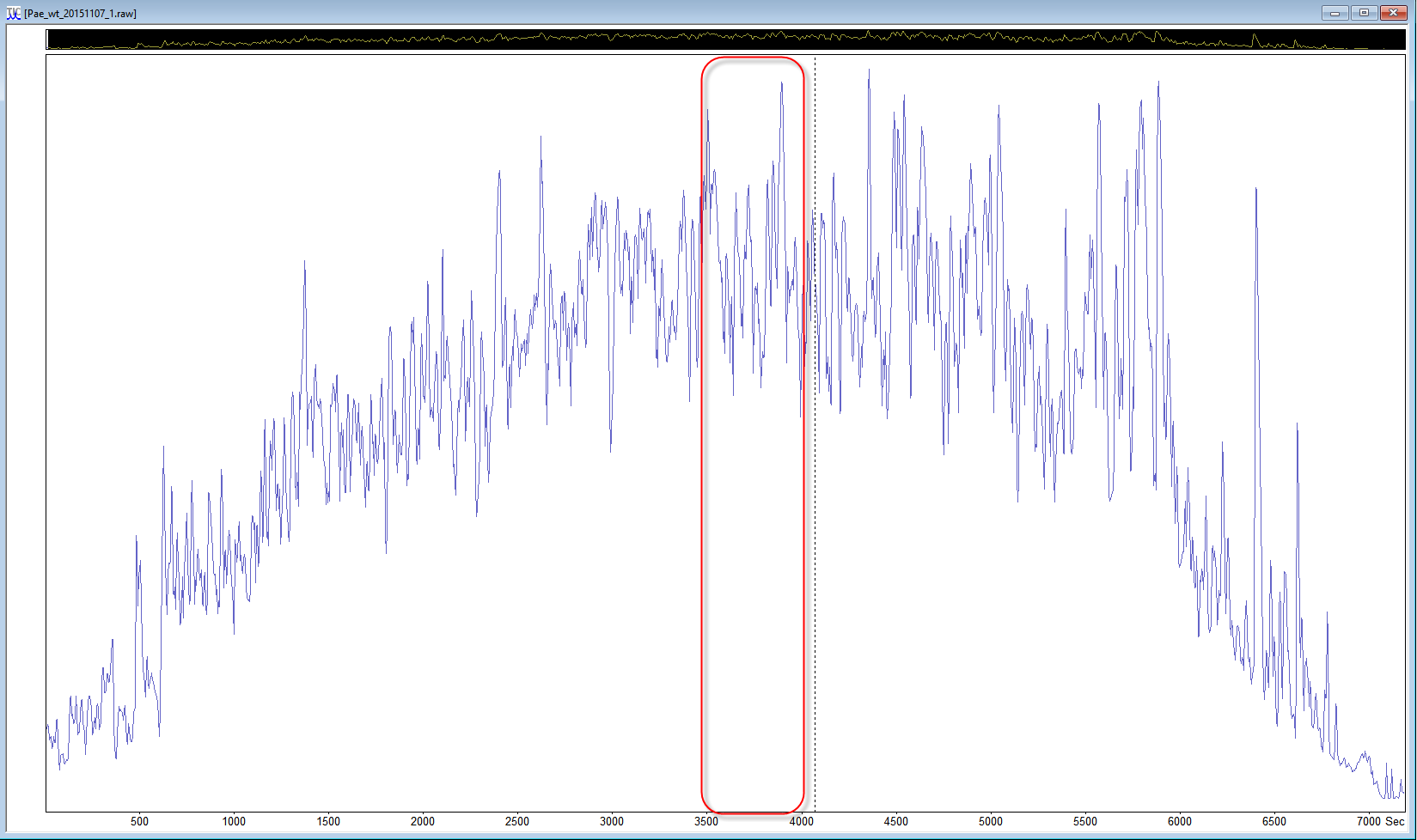
If the data set is a multi-file data set, start with just one file, and if the samples were fractionated, a file from the middle of the data set can be a better choice. If you are using Mascot Distiller, you can even reduce the size of the search to a “busy” section of a data file. Look at the TIC to choose a section in the middle of the run where there are lots of peaks and the trace is high above the baseline, and select a ~500 second region, then choose process range to create a small peak list for test purposes.
There is no real need to select a decoy search at this point. If you know the organism the sample came from and it is covered by the taxonomy filters, use that species with the Swissprot database. If the taxonomy filter covers a wider group of related species, like bacteria, try using a UniProt proteome database instead. If you don’t know the species that the sample came from, use the whole of SwissProt for the first search. I normally include a contaminants database too. The aim of this test search is to identify enough peptides with limited modifications under these search conditions so that we can start to fine tune the search parameters.
There are of course plenty of ways the initial search parameters can fail. Most of the time it is going to be due to an unexpected experimental detail such as a different enzyme or akylation agent.
3. Determine mass tolerances from results
Once the search has completed, you should see a reasonable number of matches. Expand the “Modification statistics” section to make sure there are some matches with the fixed modification you chose (Carbamidomethyl (C) in this case). If you did not know beforehand, you should now know the species for the sample. Looking at the top two or three protein hits, expand the report to see the peptide matches and click on the accession numbers to see the protein reports in a new tab. These top protein hits should have high sequence coverage, over 50% and often 80% or more. The sequence coverage is unlikely to be 100% as Mascot only looks for peptides that are 7 amino acids or longer, so there will be a number of small gaps depending on the distribution of lysine and arginine residues when using trypsin, and similarly with other enzymes.
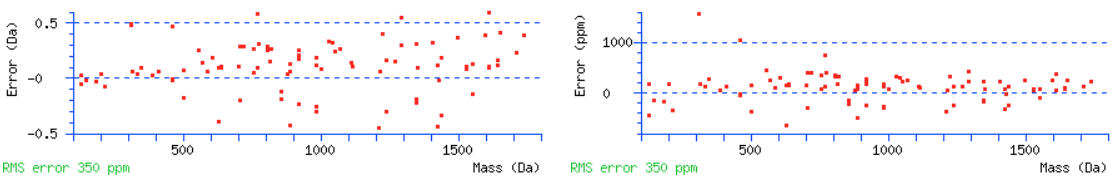
Scroll down below the peptide matches to see the precursor mass error graph. Do the majority of the peptides fall in to a narrow tolerance range? Or are the errors distributed across the mass range and look like they go off the edge of the graph? There will always be some outliers. You should be able to determine if you need a wider tolerance or if you can narrow it.
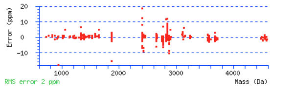
For this example, a peptide tolerance of ± 10 ppm would be a good choice.
Go back to the main report and find some high mass/long peptides with high scores. Over 100 is great but scores over 70 or so will also work. Click the query numbers and the peptide view will open in a new tab. We should see nice coverage of both b and y ions series. If there are no high scoring peptides, the data may be ETD/ECD data and you should actually be searching for c and z+1 ions. Scrolling down to the graphs, we can again estimate a suitable tolerance for the MS/MS ions. Warning signs that the tolerance needs to be wider are measured errors leading up to the edge of the graphs and having no errors for the higher mass ions.
For this data set the initial MS/MS tolerance of 0.6 Da should be fine.
4. Error tolerant search to find common modifications
Now that we have determined initial search tolerances, try researching the data as an error tolerant search with these tolerances. Use the correct taxonomy filter or a UniProt proteome database. The goal is to determine if there are unusual numbers of any particular modification or non-specific cleavages. The error tolerant search results should expose excessive deamidation, missed cleavages or abundant unsuspected modifications. You may want to skip this step if you have already included 3 or 4 variable modifications in the initial search due to the experimental design and sample preparation.
Once the error tolerant search is complete, expand the “Modification statistics” section to see the counts. Our advice is to only select the most abundant one to two unsuspected modifications as variable modifications in the optimized search. If you select too many variable modifications, over 4 or so, the search conditions will cause a combinatorial explosion of modification site permutations, which increases the search space. The search will both take a very long time and lose sensitivity such that you will actually end up with worse results.
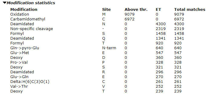
In our example search, we can see high counts for deamidation and formylation. When evaluating modifications to include, look at the ratio of the modified matches to the total number of matches. For formylation this comes out at about 5% and we should include it. The proportion will be higher in the optimized search as the long tail of less abundant modifications will not be included. I chose not to include the Gln->pyro-Glu in the final search although it is a reasonable candidate and, due to its specificity, would not expand the search space too much. However, it accounted for less than 1% of the matches in the error tolerant search.
There are quite a lot of non-specific cleavages identified. Looking at the error tolerant results, I can see that most really are non-specific, so increasing the number of missed cleavages will not increase the number of matches very much and I am not willing to give up the enzyme specificity.
5. Putting it all together for the final analysis
We are now ready to run the optimized search. It’s time to include a decoy in the search. Once the search completes, check the False Discovery Rate and adjust to 1%. Compare the number of matches above the thresholds to the total number of queries submitted. Total query identification rates vary from 5% up to 50% plus depending on the data set. It came out at 34% for this search. The Deamidated and Formyl modifications accounted for 17% and 7% of the total matches respectively so they were worth including. If everything looks good, go ahead and analyze the complete data set.
Keywords: error tolerant, tutorial